Xenium mouse brain

In this notebook, we will use ovrlpy to investigate the Xenium’s mouse brain dataset.

We want to create a signal embedding of the transcriptome, and a vertical signal incoherence map to identify locations with a high risk of containing spatial doublets.

We want to create a signal embedding of the transcriptome, and a vertical signal incoherence map to identify locations with a high risk of containing spatial doublets.

Settings and Imports

First we import relevant analysis packages and set the paths to the data files.

from pathlib import Path

import matplotlib.pyplot as plt
import numpy as np
import pandas as pd

import ovrlpy

data_path = Path(
    "/dh-projects/ag-ishaque/raw_data/tiesmeys-ovrlpy/Xenium-brain-2024/replicate1"
)

signature_matrix_file = Path(
    "/dh-projects/ag-ishaque/raw_data/Xenium-benchmark/scRNAseq/trimmed_means.csv"
)

result_folder = Path("results")
result_folder.mkdir(exist_ok=True, parents=True)

Loading the data

Now, we want to load the data and prepare it for analysis.

coordinate_df = ovrlpy.io.read_Xenium(data_path / "transcripts.parquet")

coordinate_df.head()

	gene	x	y	z
0	Bhlhe40	4843.045898	6427.729980	19.068869
1	Parm1	4844.632812	6223.182617	18.520161
2	Bhlhe40	4842.943359	6478.310547	18.500109
3	Lyz2	4843.941406	6344.550293	15.016154
4	Dkk3	4843.162598	6632.111816	15.394680

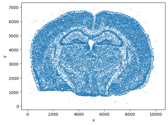
Let’s get a quick overview of the tissue

_ = coordinate_df[::1000].plot.scatter(x="x", y="y", s=0.1)

Running the ovrlpy pipeline

ovrlpy provides a convenience function run to run the entire pipeline. The function creates a signal integrity map, a signal strength map and a Visualizer obejcet to visualize the results.

signal_integrity, signal_strength, visualizer = ovrlpy.run(
    df=coordinate_df, cell_diameter=10, n_expected_celltypes=30, n_workers=8
)

Running vertical adjustment
Creating gene expression embeddings for visualization:
Analyzing in 3d mode:
determining pseudocells:
found 62341 pseudocells
sampling expression:

100%|██████████| 88/88 [02:21<00:00,  1.61s/it]

Modeling 30 pseudo-celltype clusters;
Creating signal integrity map:

 94%|█████████▍| 296/315 [06:33<00:21,  1.15s/it]/dh-projects/ag-ishaque/analysis/muellni/envs/ovrlpy/lib/python3.12/site-packages/ovrlpy/_utils.py:397: RuntimeWarning: invalid value encountered in divide
  spatial_patch_cosine_similarity[patch_signal_mask] = np.sum(
100%|██████████| 315/315 [06:41<00:00,  1.28s/it]

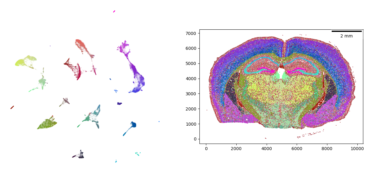
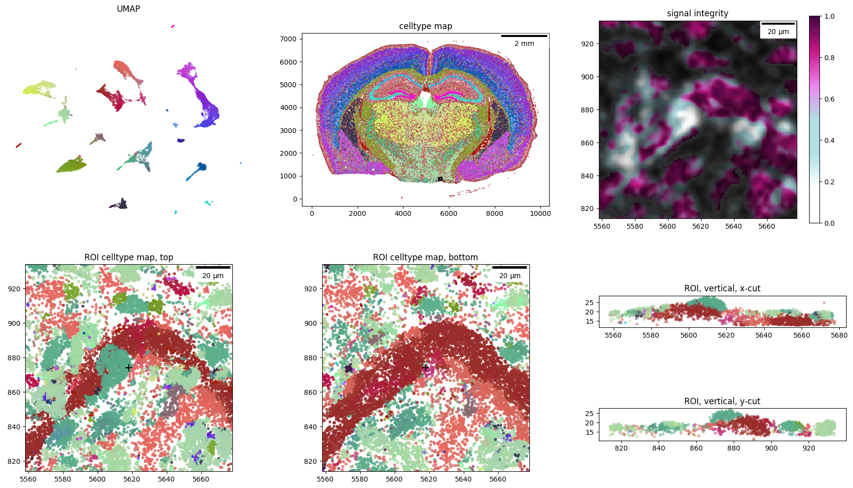
Visualizing results

The visualizer object has a plotting method to show the embeddings of the sampled gene expression signal.

visualizer.plot_fit()

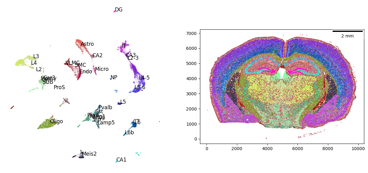
We can annotate the UMAP using external, single-cell derived cell type signatures to help interpret the cell type clusters in the gene-expression embedding:

signatures = pd.read_csv(signature_matrix_file, index_col=0).T.loc[
    :, lambda df: df.columns.isin(visualizer.genes)
]

signatures = signatures.groupby(
    lambda x: x.split("_")[1].split(" ")[0].split("-")[0]
).mean()

signatures.index = signatures.index.str.replace("/", "-")
signatures.index.name = "celltype"

signatures.iloc[:5, :5]

feature	Sox17	Col19a1	2010300C02Rik	Satb2	Nrp2
celltype
Astro	0.0	0.000000	0.000000	0.000000	1.316010
CA1	0.0	0.000000	7.463820	2.937198	0.693990
CA2	0.0	0.000000	9.586734	0.000000	2.942782
CA3	0.0	0.051941	6.305638	0.000000	6.810690
CR	0.0	0.000000	0.000000	0.000000	0.000000

visualizer.fit_signatures(signatures)
visualizer.plot_fit()

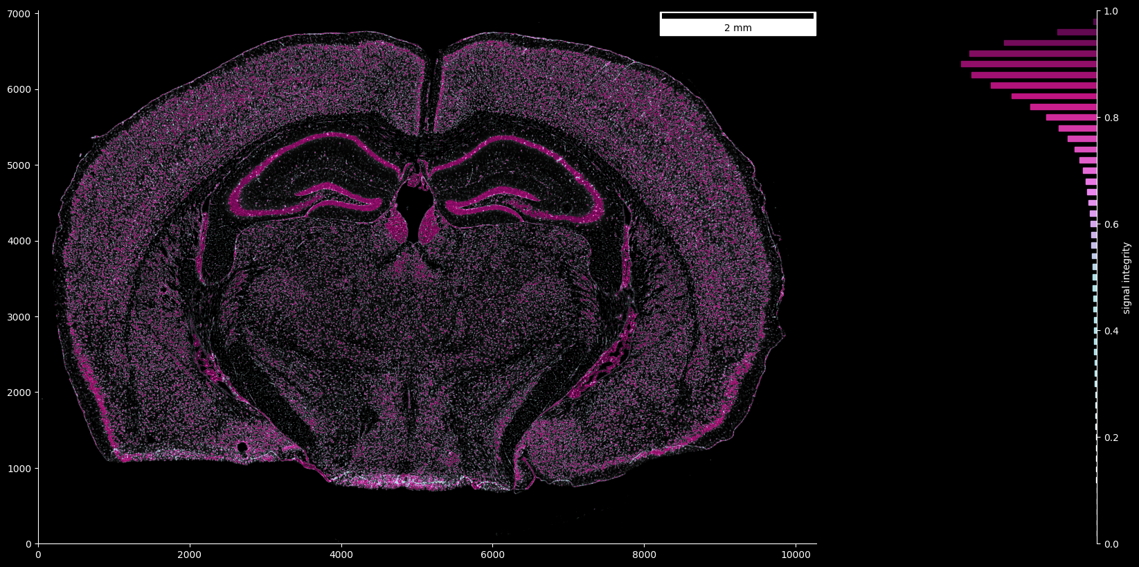
In the same way, the signal integrity map can be visualized, where visualization is cut off at regions below a certain signal strength threshold:

fig, ax = ovrlpy.plot_signal_integrity(
    signal_integrity, signal_strength, signal_threshold=3
)

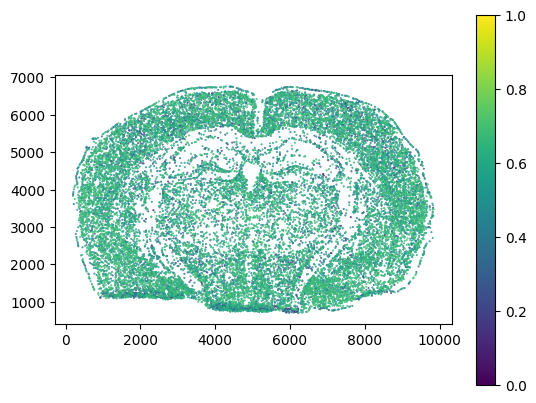
Detecting doublets

We can detect individual doublet events with ovrlpy, again setting a signal strength threshold to filter out low-transcript regions:

doublet_df = ovrlpy.detect_doublets(
    signal_integrity, signal_strength, minimum_signal_strength=3, integrity_sigma=2
)

_ = plt.scatter(
    doublet_df["x"],
    doublet_df["y"],
    c=doublet_df["integrity"],
    s=0.2,
    cmap="viridis",
    vmin=0,
    vmax=1,
)
_ = plt.gca().set_aspect("equal")
_ = plt.colorbar()

Having sampled regions of potential doublets, we can visualize them as close-up transcriptome molecule clouds through the Visualizer’s learned color embeddings - by providing their (x, y) locations to ovrlpy.plot_region_of_interest

doublet_case = 0

x, y = doublet_df.loc[doublet_case, ["x", "y"]]

_ = ovrlpy.plot_region_of_interest(
    x, y, coordinate_df, visualizer, signal_integrity, signal_strength, window_size=60
)

/dh-projects/ag-ishaque/analysis/muellni/envs/ovrlpy/lib/python3.12/site-packages/sklearn/base.py:493: UserWarning: X does not have valid feature names, but PCA was fitted with feature names
  warnings.warn(

Other functionality

Furthermore, we can save the visualizer object to file for later use leveraging the pickle module

import pickle

with open("my_analysis.pickle", "wb") as file:
    pickle.dump(visualizer, file)

… and easily reload it if needed.

with open("my_analysis.pickle", "rb") as file:
    visualizer = pickle.load(file)

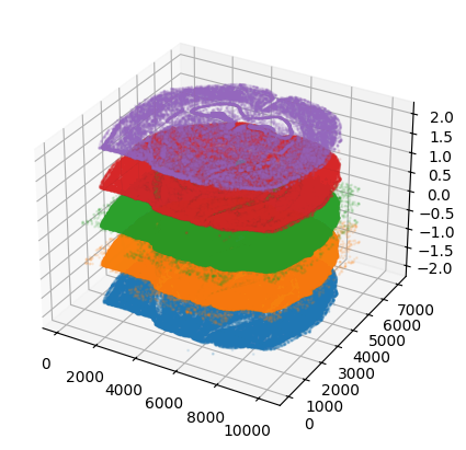
Additionally, the analysis has produced a global z-level adjustment of the transcriptome coordinates, which can be used to create a z-stack of adjacent, aligned sections in silico:

plt.figure(figsize=(20, 5))

ax = plt.subplot(111, projection="3d")

for i in range(-2, 3):
    subset = coordinate_df[(coordinate_df.z - coordinate_df.z_delim).between(i, i + 1)]

    ax.scatter(
        subset.x[::100],
        subset.y[::100],
        np.zeros(1 + (len(subset) // 100)) + i,
        s=1,
        alpha=0.1,
    )